Measuring Risk Attitudes in the Field
Risk preferences play an important role in many domains of decision-making, and heterogeneity in risk attitudes has implications for our analysis and policy recommendations. As researchers collecting data in the field, we may (in some circumstances) want to directly measure the risk attitudes of the individuals we study. In this post, we discuss some of the most popular elicitation and estimation methods for risk preferences.
There is no single optimal method; the decision on which approach to use (if any) depends on a number of factors, primarily the importance of risk preferences to our specific research question. As discussed by David McKenzie in a recent blog post,[1] there is a reasonable argument to be made for measuring various dimensions of preferences that could be important for decision-making, such as risk and time preferences, subjective expectations, altruism, trust, cognitive skills, personality traits etc. However, given time and budget constraints, we need to decide which of these are most important to our particular research question.
If we do decide to measure risk preferences, then there is a trade-off between simple measures that participants are more likely to understand and take less time to implement, and more complicated methods that allow us to estimate risk preferences more formally, for example by inferring “bounds” using simple one-parameter utility functions. We could even structurally estimate parameters of more complicated utility functions that go beyond expected utility theory (EUT) by incorporating models such as prospect theory, jointly estimating parameters for loss aversion and non-linear probability weighting. Note that “risk attitudes” can in general incorporate all three of these dimensions (utility curvature, reference-dependent preferences, non-linear probability weighting functions), but for brevity in this post we will not discuss the estimation of loss aversion or probability weighting.[2] Another thing we will not discuss is the “to incentivise or not to incentivise” debate. This decision will depend on a number of factors, including practical considerations and the importance of risk preferences in one’s research question. All of the methods below can be implemented without financial incentives, or with incentivisation by providing a financial reward to participants (for example, at the end of the session based on a randomly selected subset of their decisions; needless to say, participants can never lose any money overall). We also do not discuss joint estimation of risk and time preferences. For discussions of all of these points, and more comprehensive coverage of elicitation and estimation methods, see the excellent surveys by Harrison and Rutström (2008) and Charness, Gneezy, and Imas (2013).
- Survey-based measures. These methods ask individuals to self-report their level of risk tolerance, usually using questions of the form “rate your willingness to take risk in general”, and allowing respondents to choose a number from a 10-point scale, with 1 implying that they are completely unwilling to takes risks, and 10 as completely willing to take risk. Weber, Blais, and Betz (2002) developed a domain-specific risk-taking scale (DOSPERT) that contains many items in the financial, investment, health, social, ethical and recreational domains. A number of papers have provided evidence for the domain-specific nature of preferences, and generally for the correlation between survey-based measures and incentivised experimental measures, and the power of these measures in predicting real financial outcomes such as job choice and portfolio selection (see for example recent work by Falk, Becker, Dohmen, Enke, Huffman, and Sunde (2018), who use data from 76 countries and over 80,000 respondents as part of their Global Preferences Survey).[3] Vieider et al. (2015) also demonstrate (with evidence from 30 countries) that responses to general and financial survey questions correlate well with incentivised choices in many countries, but that the magnitude and statistical significance of the correlation varies substantively across countries. This suggests that the experimental validity of qualitative survey measures may be context-specific and sensitive to what people perceive the word “risk” to mean. We usually think of risk as objectively known probabilities, such as those controlled by experimental researchers in the lab, but this might differ a lot from people’s broader concept of risk as “uncertainty”, where the explicit probabilities of the outcome generating process are not clear.
-
A single portfolio choice question. Gneezy and Potters (1997) developed a simple measure of risk preferences, whereby subjects are allocated a gift of $X and are asked: (i) how much they wish to keep ($x); (ii) how much they wish to invest in a risky option that pays a dividend $kx (k>1) with probability p (and pays 0 with probability 1-p). For example, this can be implemented with a gift of 100 and a risky asset that returns 2.5 times the amount invested with probability 0.5. The amount invested then captures the individual’s attitude to risk. One drawback of this method is that it cannot distinguish between risk-seeking and risk-neutral behaviour.
-
Offering a single choice from a list of binary-outcome options. This was first developed by Binswanger (1980) and Eckel and Grossman (2002). Subjects are offered a choice of binary-outcome prospects (consisting of a “low” and a “high” payoff, with the probability of each usually held fixed at 0.5). Here is an illustrative example (subjects are typically not shown the “expected payoff” column):
Option
Low payoff
High payoff
Expected payoff
1
28
28
28
2
24
36
30
3
20
44
32
4
16
52
34
5
12
60
36
6
2
70
36
The first option is deterministic (low and high payoffs are the same). Subsequent options increase in expected payoff but also in the variance around that payoff (the high outcome increases by a larger amount than the low outcome decreases, relative to the previous option). Note than options 5 and 6 are designed to separate risk-neutral from risk-seeking individuals, since option 6 has the same expected payoff as option 5 but with a higher variance. One note of caution: the fact that the first option offers a certain payment may frame the choices in a way that makes them “sign dependent”, since the certain amount may provide a reference point to identify gains and losses, and so this method may conflate reference-dependent preferences with utility curvature.
4. Certainty equivalent (CE). In this method, participants are offered the choice between a risky option and a certain payment. To illustrate, consider Barr and Packard’s (2002) framing of this choice as a decision between investing in a “risky firm” or a “safe firm”:
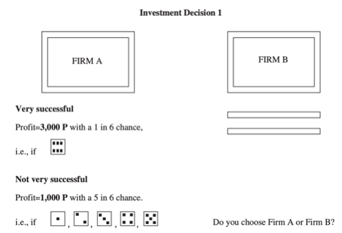
The risky firm generates a profit of 3,000 with probability1/6 and a profit of 1,000 with a probability of 5/6, while the safe firm always pays a profit of X. X begins at a low number (e.g. 1,000, which the participant would be expected to reject, as it is equal to the lowest payoff in the risky firm) and X is incrementally increased to 3,000, with participants asked to choose between the two firms each time X is changed. The certainty equivalent is the point at which participants switch from the risky firm to the safe firm. The CE activity appears to be straightforward for most people to understand (for example, it been used successfully by Vieider et al. (2015) in 30 countries), and it can provide rich data from which to estimate risk preferences. In recent work, Bauer, Chytilová, and Miguel (2019) test an unincentivised version of a similar activity and find that it correlates well with responses in the incentivised measure (and they find that the correlation is stronger than that between the incentivised version and more abstract “attitudes towards risk” survey-based questions).
5. Multiple price lists (MPL). This method, popularised by Holt and Laury (2002), is similar to the CE method, except that both options being considered are “risky”. Participants are offered a list of decisions between paired options, with each option having two outcomes, where the probabilities of each are varied. Alternative “blocks” of decisions are then offered, with the payoffs changing. This large number of decisions allows a more precise estimate of risk attitudes. However, the MPL may be relatively complicated for some subjects to understand, which affects the reliability of the estimates since parameter estimation often requires a unique “switch point” (where a subjects switches from one option to the other) and such inconsistent behaviour provides a challenge to rationalise using standard assumptions about preferences (multiple switches may also reveal indifferences between options, and some researchers do allow indifference to be expressed).
6. Willingness to pay. The Becker-DeGroot-Marschak (BDM) method asks subjects to state a minimum price to give up a prospect that they have been endowed with. Individuals are endowed with a series of risky options and asked for the “selling price”. They are told that a “buying price” will be chosen at random, and – if it is greater than the stated selling price – they will get that amount of money, otherwise they will play out the risky option. This auction-type procedure is theoretically appealing in that it provide a formal incentive for subjects to truthfully reveal their certainty equivalent, but there is a big risk that participants fail to understand the logic (in particular, that the buying price cannot be affected by what they state as the selling price).
Once we have our data on choices made by participants, the simplest thing that we could do to summarise the risk preferences would be to create an index. For example, in the CE method, we could add up the number of certain choices made by participants as an index of risk aversion, which we can then use to form a “median-split” or split into terciles. All of the aforementioned methods allow a simple way of creating such an index, but the more complex methods also allow us to formally estimate risk preferences parameters. Here we will briefly mention two estimation methods;[4] further details can be found in Harrison and Rutström (2008).
- Inferring bounds. If we are willing to assume EUT and a single-parameter utility function such as U(x)=x^r where x is wealth and r is the risk aversion parameter, then we can then infer bounds from decisions made. For example, in the “Binswanger” activity, we can calculate the value of r that would make the individual indifferent between the option they chose and the two options on either side to give us an estimate of a range. One drawback of this approach is that it doesn’t easily allow analysis with more complicated utility functions or the incorporation of non-EUT models, and results can be affected if there are errors in the data (for example, multiple switching points, or “order effects”).
- Structural estimation. Another approach is to specify some latent choice model and estimate the core risk parameter using maximum likelihood. This approach also allows us to explicitly incorporate non-EUT models in which there are several parameters defining risk attitudes. To illustrate with EUT, if we again assume a simple utility function such as U(x)=x^r, then we can calculate the expected utility (EU) of an option as the probability-weighted utility of each payoff in that option. For example, if the participants had the choice between two options: (i) one that had a payoff of 1,000 with probability of 0.5, or a payoff of 100 with probability of 0.5; (ii) the second having a payoff of 500 with probability 0.75 and an outcome of 250 with probability 0.25, we calculate the expected utility of each option for a “candidate value” of r (EU(i) and EU(ii)), and generate an index that equals the EU difference (EU(ii) – EU(i)). We can then link this latent index to the observed choices using a “link function”, such as a standard normal cumulative distribution function, which takes in any value for this index and transforms it into a number between 0 and 1. The “likelihood” of our observed responses then depends on the estimates of r in this specification, and we can write down a log-likelihood function and estimate the parameter r using maximum likelihood. The method can easily be extended to calculate the “prospective utility”, if we specify a model with a loss aversion parameter and / or a probability weighting function, as well as extensions to allow “stochastic errors” in decision making, and to estimate “mixture models” that allow both EUT and prospect theory (as well as other models) to be latent decision-making processes generating the observed choices, rather than choosing just one model.
The advantages of complicated elicitation methods may be outweighed by lower comprehension and nosier data. As discussed by Charness and Viceisza (2015), the commonly found lack of comprehension in methods such as MPL poses significant challenges for our ability to make policy recommendations, especially if differing comprehension levels correlate with differences in preferences. If elicitation tasks are mostly picking up “noise”, then it has serious implications for estimation and inference. Having said that, not all tasks actually allow one to detect a lack of comprehension, so the extra complication of certain elicitation methods (and the ability to explicitly capture misunderstanding, such as with ‘multiple switches’) may actually be a feature rather than a bug.[5] A final point to note is on the stability of preferences. Even if we assume that we can account for variation in elicited preferences due to noise, there is also a question about whether preferences are stable over time (and whether we should even expect them to be). Chuang and Schechter (2015) present a comprehensive review of the literature on preference stability and the effects of shocks.[6] To conclude, for a specific research project, piloting of different methods is advisable, to understand how long the method will take to implement, how well people understand it, the variation we get in the data, how results looks compared to other studies, and the correlation in the resulting measures of risk attitudes if we test multiple methods. Researchers should then choose the method that is best suited to their sample population and questions of interest.
[1] https://blogs.worldbank.org/impactevaluations/weekly-links-june-7-should-we-elicit-preferences-more-and-better-collider-bias
[2] While risk aversion is usually thought of as curvature of the utility function, it is actually possible – outside of the Expected Utility theory framework – for an individual to display “risk averse behaviour” while having a linear or even convex utility function (risk aversion would in that case work through probability weighting or loss aversion; see Yaari (1987)). Tanaka, Camerer, and Nguyen (2010) is one example of an attempt to jointly measure loss aversion and risk aversion (as well as time preferences) in a developing country setting.
[3] https://www.briq-institute.org/global-preferences/about
[4] There are also non-parametric methods for estimating risk preferences (see for example, Hey and Orme, 1994; Wakker and Deneffe, 1996; Abdellaoui, Bleichrodt, and Paraschiv, 2007).
[5] Thanks to Amma Panin for pointing this out.
[6] Also see Jakiela and Ozier (2019) for the effect of shocks on risk preferences.
Abdellaoui, M., Bleichrodt, H., & Paraschiv, C. (2007). Loss aversion under prospect theory: A parameter-free measurement. Management Science, 53(10), 1659-1674.
Bauer, M., Chytilová, J., & Miguel, E. (2019). Using Survey Questions to Measure Preferences: Lessons from an Experimental Validation in Kenya.
Charness, G., Gneezy, U., & Imas, A. (2013). Experimental methods: Eliciting risk preferences. Journal of Economic Behavior & Organization, 87, 43-51.
Charness, G., & Viceisza, A. (2015). Three risk-elicitation methods in the field: Evidence from rural Senegal.
Chuang, Y., & Schechter, L. (2015). Stability of experimental and survey measures of risk, time, and social preferences: A review and some new results. Journal of Development Economics, 117, 151-170.
Falk, A., Becker, A., Dohmen, T., Enke, B., Huffman, D., & Sunde, U. (2018). Global evidence on economic preferences. The Quarterly Journal of Economics, 133(4), 1645-1692.
Gneezy, U., & Potters, J. (1997). An experiment on risk taking and evaluation periods. The Quarterly Journal of Economics, 112(2), 631-645.
Harrison, G. W., & Elisabet Rutström, E. (2008). Risk aversion in the laboratory. In Risk aversion in experiments (pp. 41-196). Emerald Group Publishing Limited.
Hey, J. D., & Orme, C. (1994). Investigating generalizations of expected utility theory using experimental data. Econometrica: Journal of the Econometric Society, 1291-1326.
Holt, C. A., & Laury, S. K. (2002). Risk aversion and incentive effects. American Economic Review, 92(5), 1644–1655.
Jakiela, P., & Ozier, O. (2019). The impact of violence on individual risk preferences: evidence from a natural experiment. Review of Economics and Statistics, 101(3), 547-559.
Tanaka, T., Camerer, C. F., & Nguyen, Q. (2010). Risk and time preferences: Linking experimental and household survey data from Vietnam. American Economic Review, 100(1), 557-71.
Vieider, F. M., Lefebvre, M., Bouchouicha, R., Chmura, T., Hakimov, R., Krawczyk, M., & Martinsson, P. (2015). Common components of risk and uncertainty attitudes across contexts and domains: Evidence from 30 countries. Journal of the European Economic Association, 13(3), 421-452.
Wakker, P., & Deneffe, D. (1996). Eliciting von Neumann-Morgenstern utilities when probabilities are distorted or unknown. Management science, 42(8), 1131-1150.
Yaari, M. E. (1987). The dual theory of choice under risk. Econometrica, 55(1), 95–115.